Spectral discretization

This document explains how the spectral domain is discretize in Eradiate simulations.

Note

This section assumes that you are familiar with Experiment objects.

Depending on the active mode, the spectral discretization has a different meaning:

• In monochromatic mode, the spectral discretization is specified by a WavelengthSet, i.e. an array of wavelengths.

• In CKD mode, the spectral discretization is specified by a BinSet, i.e. a set of CKD bins.

An Experiment has as many spectral discretizations as it has measures.

In both modes, the spectral discretization corresponding to each measure is determined in three steps:

1. The spectral discretization is set to the Experiment default spectral discretization, which is controlled by the default_spectral_set parameter.

2. If an atmosphere is present, this default spectral set may be replaced by a spectral set specific to the atmosphere. Typically, it is specified by its absorption dataset when the atmosphere is molecular and absorbing.

3. A subset of the default spectral set is finally selected depending on the measure’s spectral response response.

Hereafter we illustrate the spectral discretization building process in common use cases with AtmosphereExperiment. The below modules will be required all along; let us import them once for all:

import numpy as np

import eradiate

from eradiate.experiments import AtmopshereExperiment
from eradiate import unit_registry as ureg

The following sections are organized based on

• the Eradiate active mode

• the presence of an atmosphere, namely an absorbing molecular atmosphere

• the desired spectral discretization type, i.e. either a wavelength interval or a set of isolated wavelengths/bins.

Note

All atmosphere are not necessarily overriding the experiment’s spectral set, but absorbing molecular atmosphere are. This is because atmospheric absorption spectra are generally the highest varying spectra in the entire scene. For best accuracy, one must use a spectral discretization that is fine enough to capture these absorption features. As such, the spectral discretization associated to the atmospheric absorption spectra takes precedence over other spectral discretization.

Monochromatic mode

eradiate.set_mode("mono")

from eradiate.spectral import WavelengthSet

Without atmosphere

In a wavelength interval

This use case is typically encountered when the user wants to perform a monochromatic simulation in the wavelength interval corresponding to the spectral band of a given satellite instrument. In this case, the user can simply set the srf attribute to the identifier corresponding to the platform, instrument and spectral band.

Example

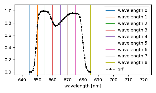
The following example illustrates how to perform a monochromatic simulation in the wavelength interval corresponding to the 4th spectral band of the MSI instrument onboard the Sentinel 2A platform, which extends from 645 nm to 685 nm. We set the experiment’s default_spectral_set parameter so that the simulation is run ever 5 nm. To increase or decrease this spectral discretization, the user should set this attribute to a different value. If unset, a spectral discretization of 1 nm is used, by default.

exp = AtmosphereExperiment(
  default_spectral_set=WavelengthSet.arange(
      645.0 * ureg.nm,
      686.0 * ureg.nm,
      5.0 * ureg.nm,
  ),
  atmosphere=None,
  measures={
    "type": "multi_distant",
    "srf": "sentinel_2a-msi-4",
  }
)

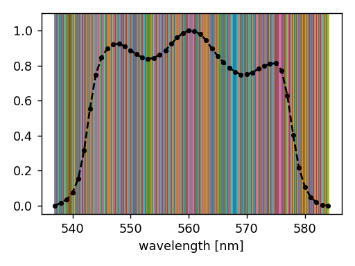
The resulting wavelength set is illustrated below, superimposed on the spectral response function of the 4th band of the MSI instrument.

If you want to perform a monochromatic simulation in an arbitrary wavelength interval, use an InterpolatedSpectrum to define a generic spectral response function that covers that interval.

Example

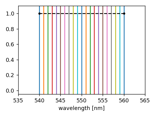
The following example illustrates how to perform a monochromatic simulation in the (arbitrary) wavelength interval [540, 560] nm.

exp = AtmosphereExperiment(
  atmosphere=None,
  measures={
    "type": "multi_distant",
    "srf": {
      "type": "interpolated",
      "wavelengths": np.array([540.0, 560.0]) * ureg.nm,
      "values": np.array([1.0, 1.0]),
    },
  }
)

Since we did not set the default_spectral_set attribute, the simulation is run every 1 nm from 540 nm to 560 nm.

At isolated wavelength(s)

The recommended way to achieve this is to use a MultiDeltaSpectrum to define the spectral response function of the associated measure. The wavelengths at which the simulation is performed are then specified by the wavelengths attribute.

Example

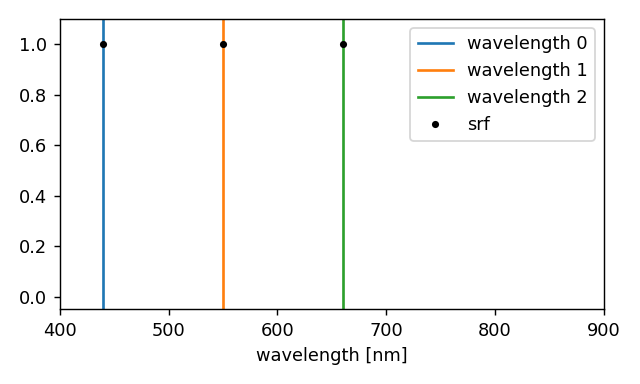
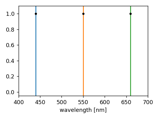
The following example illustrates how to perform a monochromatic simulation at 440 nm, 550 nm and 660 nm.

exp = AtmosphereExperiment(
  atmosphere=None,
  measures={
    "type": "multi_distant",
    "srf": {
      "type": "multi_delta",
      "wavelengths": np.array([440.0, 550.0, 660.0]) * ureg.nm,
    },
  }
)

With atmosphere

When an absorbing molecular atmosphere is present, the Experiment default wavelength set is replaced by that of the atmosphere’s absorption dataset.

In a wavelength interval

Example

The following example illustrates how to perform a monochromatic simulation in the 3rd band of the MSI instrument onboard the Sentinel 2A platform.

We first prepare the monochromatic absorption dataset in the interval [537, 584] nm, corresponding to the 3rd band of the MSI instrument onboard the Sentinel 2A platform:

import xarray as xr

from eradiate import data
from eradiate.radprops._util_mono import get_us76_u86_4_spectrum_filename

path2 = get_us76_u86_4_spectrum_filename(537 * ureg.nm)
path1 = get_us76_u86_4_spectrum_filename(584 * ureg.nm)
ds1 = data.load_dataset(path1)
ds2 = data.load_dataset(path2)

ds = xr.concat([ds1.isel(w=slice(0,-1)), ds2], dim="w")

The experiment is created with:

exp = AtmosphereExperiment(
  atmosphere={
    "type": "molecular",
    "construct": "ussa_1976",
    "absorption_dataset": ds
  },
  measures={
    "type": "multi_distant",
    "srf": "sentinel_2a-msi-3",
  }
)

Inspection of exp.spectral_set will show that the wavelength set includes more than 100 thousands of wavelengths, as illustrated below.

Running such a simulation will take a long time (10 hours order of magnitude). This explains why the CKD mode is recommended for this use case.

Another way is to downsample the absorption dataset to a coarser spectral grid, so that the corresponding spectral set is smaller. However, one must be careful with this approach, as downsampling the absorption dataset may lead to a significant loss of accuracy in the simulation results.

At isolated wavelength(s)

Example

The following example illustrates how to perform a monochromatic simulation at 560 nm.

exp = AtmosphereExperiment(
  atmosphere={
    "type": "molecular",
    "construct": "ussa_1976",
    "absorption_dataset": ds,
  },
  measures={
    "type": "multi_distant",
    "srf": {
      "type": "multi_delta",
      "wavelengths": [440, 550.0, 660.0] * ureg.nm,
    },
  }
)

In this case, the spectral set has been reduced to a single wavelength.

CKD mode

eradiate.set_mode("ckd")

from eradiate.spectral import BinSet

Without atmosphere

In a wavelength interval

Similarly to the monochromatic mode, the user can specify a wavelength interval to perform the simulation in, either by specifying a platform, an instrument and the spectral band, or by defining an arbitrary spectral response function.

Example

Below, we create an experiment that performs a simulation in the 3rd band of the MSI instrument onboard the Sentinel 2A platform.

exp = AtmosphereExperiment(
  atmosphere=None,
  measures={
    "type": "multi_distant",
    "srf": "sentinel_2a-msi-3",
  }
)

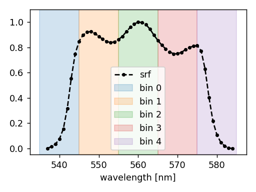
The spectral set consists of 5 bins that cover the wavelength interval from 535 nm to 585 nm (each bin is 10 nm wide), as illustrated below.

At isolated CKD bins

To select individual CKD bin(s), the MultiDeltaSpectrum is useful. It is going to select only the CKD bin(s) that include(s) each of the MultiDeltaSpectrum object’s wavelengths.

Example

The following example illustrates how to perform a CKD simulation in the CKD bins that include 560 nm and 620 nm.

exp = AtmosphereExperiment(
  atmosphere=None,
  measures={
    "type": "multi_distant",
    "srf": {
      "type": "multi_delta",
      "wavelengths": [560.0, 620.0]  * ureg.nm,
    },
  }
)

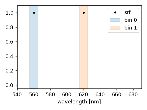
The spectral set consists of two CKD bins that covers the wavelength interval from 555 nm to 565 nm and from 615 nm to 625 nm, as illustrated below.

With atmosphere

When an absorbing molecular atmosphere is present, the Experiment default bin set is replaced by that of the atmosphere’s absorption dataset. Note that the selected CKD bin will originate from the absorption dataset, not from the experiment default bin set.

In a wavelength interval

Example

  exp = AtmosphereExperiment(
    atmosphere={
      "type": "molecular",
      "construct": "afgl_1986",
      "binset": "1nm",  # each bin is 1 nm wide
    },
  measures={
    "type": "multi_distant",
    "srf": "sentinel_2a-msi-3"
  }
)

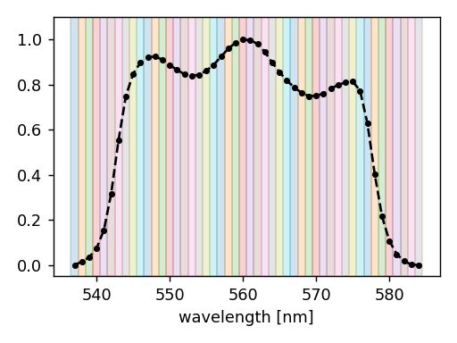
The spectral set consists of 48 bins that cover the wavelength interval
from 536.5 nm to 584.5 nm (each bin is 1 nm wide), as illustrated below.

At isolated CKD bins

To select individual CKD bin, the MultiDeltaSpectrum is useful. It is going to select only the CKD bin(s) that include(s) each of the MultiDeltaSpectrum object’s wavelengths. Note that the selected CKD bin will originate from the absorption dataset, not from the experiment default bin set.

Example

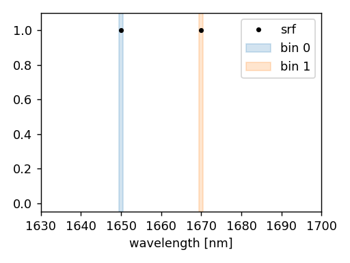
The following example illustrates how to perform a CKD simulation in the CKD bin around 560 nm.

exp = AtmosphereExperiment(
  atmosphere={
    "type": "molecular",
    "construct": "afgl_1986",
    "binset": "1nm",  # each bin is 1 nm wide
  },
  measures={
    "type": "multi_distant",
    "srf": {
      "type": "multi_delta",
      "wavelengths": [1650.0, 1670.0] * ureg.nm,
    },
  }
)

The spectral set consists of two individual bins that cover the wavelength intervals from 1649.5 nm to 1650.5 nm and from 1669.5 nm to 1670.5 nm (each bin is 1 nm wide).