[1]:
%reload_ext eradiate.notebook.tutorials
Last updated: 2023-06-22 19:50 (eradiate v0.23.2rc2.post1.dev5+gedede817.d20230622)
Filter a spectral response function#
Overview
This tutorial explains how to filter a spectral response function dataset and use the filtered dataset into an Eradiate experiment.
What you will learn
What are the reasons to filter spectral response function datasets.
How to filter a spectral response function dataset using different filtering algorithms.
What are the caveats of some filtering algorithms.
How to use the filtered spectral response function dataset in an
Experiment.
Why filter?#
This utility lets one filter spectral response function data sets. The reason for doing that could be to:
reduce the size of the data set by removing irrelevant data, e.g., leading or trailing zeros
reach a better simulation speed-versus-accuracy tradeoff, since some spectral response functions feature a very large spectral span
The eradiate.srf_tools module defines different algorithms that can be used to filter spectral response function accordingly.
These are made available through the eradiate command-line interface via the eradiate srf command group.
Although both the Python API or the CLI may be used to filter the spectral reponse function, this tutorial focuses on the Python API usage. Refer to the Command-line interface reference for more information on the CLI.
Warning
There is no universal filter algorithm. Each filter algorithm has its pros and cons. It must be stressed that using filtered spectral response function data sets will inevitably lead to less accurate results. As a result, choosing and configuring the filters must be done with great care. The filter choice and configuration is the entire reponsibility of the user.
Note
The examples below feature the spectral response functions of bands 1 and 14 of the MODIS instrument onboard the AQUA platform, downloaded on 2022-05-02 at https://oceancolor.gsfc.nasa.gov/docs/rsr/aqua_modis_RSR.nc.
They are made available at $ERADIATE_SOURCE_DIR/resources/data/tutorials/spectra/srf/.
Let us load the example datasets:
[2]:
import eradiate

aqua_modis_1 = eradiate.data.load_dataset("tutorials/spectra/srf/aqua-modis-1.nc")
aqua_modis_14 = eradiate.data.load_dataset("tutorials/spectra/srf/aqua-modis-14.nc")
Trimming#
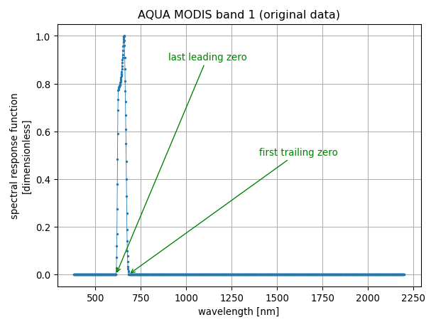
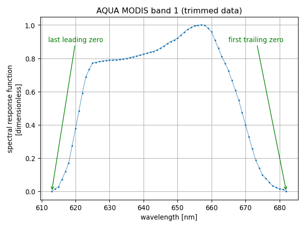
We refer to trimming as the undestructive filter that removes irrelevant leading and trailing zeros from the data set. In this regard, it can be regarded as a safe filtering algorithm.
The process of trimming is illustrated with the two figures below:
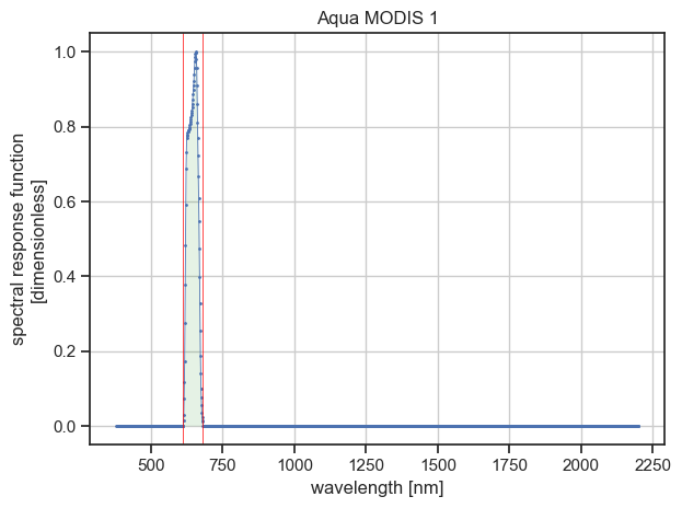
To trim a spectral response function data set, call the trim_and_save() method.
Let us call it using the parameters:
verbose=True: will display a filtering summary tableshow_plot=True: will display a figure emphasizing the filtered regiondry_run=True: will not save the trimmed dataset to the disk
[3]:
from eradiate.srf_tools import trim_and_save

trimmed = trim_and_save(
    srf=aqua_modis_1,
    path="/home/aqua-modis-1-trimmed.nc",
    verbose=True,
    show_plot=True,
    dry_run=True,
)
                      Filtering summary
┏━━━━━━━━━━━━━━━━━━━━━━━━┳━━━━━━━━━━━┳━━━━━━━━━━┳━━━━━━━━━━━━┓
┃ Characteristic         ┃  Initial  ┃  Final   ┃ Difference ┃
┡━━━━━━━━━━━━━━━━━━━━━━━━╇━━━━━━━━━━━╇━━━━━━━━━━╇━━━━━━━━━━━━┩
│ Lower wavelength       │ 380.0 nm  │ 613.0 nm │  233.0 nm  │
│ Upper wavelength       │ 2199.0 nm │ 682.0 nm │ -1517.0 nm │
│ # wavelength           │   1820    │    70    │   -1750    │
│ Wavelength range width │ 1819.0 nm │ 69.0 nm  │ -1750.0 nm │
│ Wavelength bandwidth   │  42.8 nm  │ 42.8 nm  │   0.0 nm   │
│ Mean wavelength        │ 645.8 nm  │ 645.8 nm │   0.0 nm   │
└────────────────────────┴───────────┴──────────┴────────────┘
Would write filtered data to /home/aqua-modis-1-trimmed.nc
In our example, we use the spectral response function of the band 1 of the MODIS instrument onboard the AQUA platform. The summary table (above) indicates that the spectral response function is non-zero only in the wavelength range from 613 nm to 682 nm and that to discard the data where the spectral response is zero, 1750 data points have been removed, resulting in 70 remaining data points.
The last line of the output tells us where the filtered data would have been written if we had not used dry_run=True.
Filtering#
The filter() method provides additional ways to filter spectral reponse function data sets in a way that may lead to loss of relevant data (i.e. data points where the response is non-zero).
Three filtering algorithms are defined that can be combined together:
the threshold filter: data points where response is less than or equal to a given threshold value are dropped.
the spectral filter: data points falling out of a given wavelength range are dropped.
the integral filter: data points that do not contribute to a given percentage of the integrated spectral response are dropped.
To select either one filter, simply provide the corresponding parameter(s) to filter(). For example, passing percentage=98.0 will enable the integral filter. You can pass parameters corresponding to multiple filters.
Note
By default, the filter() method trims the data set before applying the other
filters. Therefore, without any other parameter the behaviour of filter() is
equivalent to trim_and_save().
To disable the trimming step, use prior_trim=False.
Note
The filter() method provides the verbose, dry_run and interactive
parameters with the same behaviour as with the trim_and_save() method.
Threshold filter#
Use the threshold filter to discard all data points where the response is less than or equal to a given threshold value specified by the threshold parameter.
For example, to set the threshold value at 1e-3:
[4]:
from eradiate.srf_tools import filter_srf

filtered = filter_srf(
    srf=aqua_modis_14,
    path="/home/aqua-modis-14-filtered.nc",
    threshold=1e-3,
    verbose=True,
    show_plot=True,
    dry_run=True,
)
                      Filtering summary
┏━━━━━━━━━━━━━━━━━━━━━━━━┳━━━━━━━━━━━┳━━━━━━━━━━┳━━━━━━━━━━━━┓
┃ Characteristic         ┃  Initial  ┃  Final   ┃ Difference ┃
┡━━━━━━━━━━━━━━━━━━━━━━━━╇━━━━━━━━━━━╇━━━━━━━━━━╇━━━━━━━━━━━━┩
│ Lower wavelength       │ 380.0 nm  │ 654.0 nm │  274.0 nm  │
│ Upper wavelength       │ 2199.0 nm │ 697.0 nm │ -1502.0 nm │
│ # wavelength           │   1820    │    44    │   -1776    │
│ Wavelength range width │ 1819.0 nm │ 43.0 nm  │ -1776.0 nm │
│ Wavelength bandwidth   │  11.5 nm  │ 11.5 nm  │  -0.1 nm   │
│ Mean wavelength        │ 678.5 nm  │ 677.6 nm │  -0.9 nm   │
└────────────────────────┴───────────┴──────────┴────────────┘
Would write filtered data to /home/aqua-modis-14-filtered.nc
In some cases, the threshold filter might disconnect the wavelength space into two or more parts, which is often undesirable.
In such a case, a warning will appear in the command output.
This case is encountered in our example if we used the threshold value of 1e-4:
[5]:
filtered = filter_srf(
    srf=aqua_modis_14,
    path="/home/aqua-modis-14-filtered.nc",
    threshold=1e-4,
    verbose=True,
    show_plot=True,
    dry_run=True,
)
/Users/leroyv/Documents/src/rayference/rtm/eradiate/src/eradiate/srf_tools.py:514: UserWarning: Filtering this data set with threshold value of 0.0001 would disconnect the wavelength space. You probably do not want that.
  warnings.warn(
                       Filtering summary
┏━━━━━━━━━━━━━━━━━━━━━━━━┳━━━━━━━━━━━┳━━━━━━━━━━━┳━━━━━━━━━━━━┓
┃ Characteristic         ┃  Initial  ┃   Final   ┃ Difference ┃
┡━━━━━━━━━━━━━━━━━━━━━━━━╇━━━━━━━━━━━╇━━━━━━━━━━━╇━━━━━━━━━━━━┩
│ Lower wavelength       │ 380.0 nm  │ 603.0 nm  │  223.0 nm  │
│ Upper wavelength       │ 2199.0 nm │ 1064.0 nm │ -1135.0 nm │
│ # wavelength           │   1820    │    359    │   -1461    │
│ Wavelength range width │ 1819.0 nm │ 461.0 nm  │ -1358.0 nm │
│ Wavelength bandwidth   │  11.5 nm  │  11.5 nm  │   0.0 nm   │
│ Mean wavelength        │ 678.5 nm  │ 678.6 nm  │   0.1 nm   │
└────────────────────────┴───────────┴───────────┴────────────┘
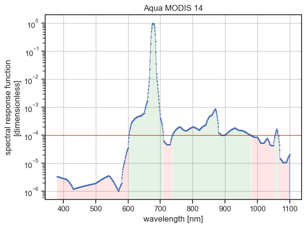
Would write filtered data to /home/aqua-modis-14-filtered.nc
The figure above illustrates that the wavelength space would be disconnected into three parts.
Note that in that case, the filtering summary table printed with --verbose does not provide information about the intermediate wavelength data points loss.
One solution to this problem is to combine the threshold filter with the spectral filter.
Spectral filter#
Use the spectral filter to discard all data points falling below or above a lower and upper wavelength, respectively, specified with the wmin, wmax parameters.
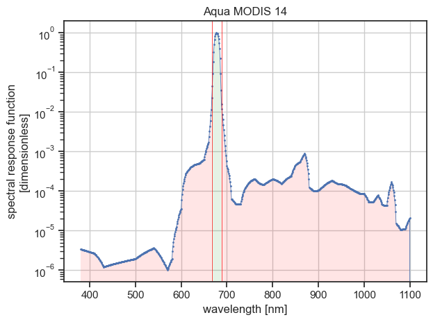
For example, to select only data within the wavelength range from 660 nanometer to 690 nanometer, enter:
[6]:
from eradiate import unit_registry as ureg

filtered = filter_srf(
    srf=aqua_modis_14,
    path="/home/aqua-modis-14-filtered.nc",
    wmin=660 * ureg.nm,
    wmax=690 * ureg.nm,
    verbose=True,
    show_plot=True,
    dry_run=True,
)
                      Filtering summary
┏━━━━━━━━━━━━━━━━━━━━━━━━┳━━━━━━━━━━━┳━━━━━━━━━━┳━━━━━━━━━━━━┓
┃ Characteristic         ┃  Initial  ┃  Final   ┃ Difference ┃
┡━━━━━━━━━━━━━━━━━━━━━━━━╇━━━━━━━━━━━╇━━━━━━━━━━╇━━━━━━━━━━━━┩
│ Lower wavelength       │ 380.0 nm  │ 660.0 nm │  280.0 nm  │
│ Upper wavelength       │ 2199.0 nm │ 690.0 nm │ -1509.0 nm │
│ # wavelength           │   1820    │    31    │   -1789    │
│ Wavelength range width │ 1819.0 nm │ 30.0 nm  │ -1789.0 nm │
│ Wavelength bandwidth   │  11.5 nm  │ 11.4 nm  │  -0.1 nm   │
│ Mean wavelength        │ 678.5 nm  │ 677.6 nm │  -1.0 nm   │
└────────────────────────┴───────────┴──────────┴────────────┘

Would write filtered data to /home/aqua-modis-14-filtered.nc
Integral filter#
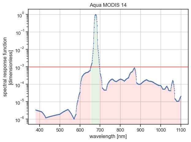
Use this filter to filter the data points based on whether they contribute to a given percentage of the integrated spectral reponse. For example, select the data points contributing to at least 98 % of the integrated spectral response with:
[7]:
filtered = filter_srf(
    srf=aqua_modis_14,
    path="/tmp/aqua-modis-14-filtered.nc",
    percentage=98.0,
    verbose=True,
    show_plot=True,
    dry_run=False,
)
                      Filtering summary
┏━━━━━━━━━━━━━━━━━━━━━━━━┳━━━━━━━━━━━┳━━━━━━━━━━┳━━━━━━━━━━━━┓
┃ Characteristic         ┃  Initial  ┃  Final   ┃ Difference ┃
┡━━━━━━━━━━━━━━━━━━━━━━━━╇━━━━━━━━━━━╇━━━━━━━━━━╇━━━━━━━━━━━━┩
│ Lower wavelength       │ 380.0 nm  │ 667.0 nm │  287.0 nm  │
│ Upper wavelength       │ 2199.0 nm │ 688.0 nm │ -1511.0 nm │
│ # wavelength           │   1820    │    22    │   -1798    │
│ Wavelength range width │ 1819.0 nm │ 21.0 nm  │ -1798.0 nm │
│ Wavelength bandwidth   │  11.5 nm  │ 11.3 nm  │  -0.2 nm   │
│ Mean wavelength        │ 678.5 nm  │ 677.6 nm │  -0.9 nm   │
└────────────────────────┴───────────┴──────────┴────────────┘
Writing filtered data to /tmp/aqua-modis-14-filtered.nc
On the figure above, the left and right red filled areas each represent 1 % or less of the integrated spectral response (mind the logarithmic scale for the ordinate axis).
Integration in Experiment#
After you filtered a spectral response function, you can use the filtered data set in any Experiment.
Simply provide the path to the filtered data set to the srf parameter in the spectral configuration of the measure scene element of your experiment.
[8]:
from eradiate.scenes.measure import MultiDistantMeasure

eradiate.set_mode("ckd")

measure = MultiDistantMeasure(
    srf="/tmp/aqua-modis-14-filtered.nc",
)