Go to notebook file

---

%reload_ext eradiate.notebook.tutorials

Last updated: 2024-03-07 15:49 (eradiate v0.25.1.dev31+g2a83b0ba.d20240229)

First steps with Eradiate

Overview

This tutorial introduces Eradiate and its approach to setting up and running simulations in a practical way.

Prerequisites

• A working installation of Eradiate (see Installation).

• Basic knowledge of the Python programming language.

This tutorial does not require prior knowledge of Eradiate.

What you will learn

• How to set up and run a simulation.

• How to visualise simulation results.

---

Importing modules

We start by importing the eradiate module. We also import a few utility libraries:

• the Numpy scientific library for array computation;

• Matplotlib’s pyplot interface to visualise our results.

import eradiate
import numpy as np
import matplotlib.pyplot as plt

We can now select an operational mode and add some aliases to submodules of Eradiate for convenience.

We will perform monochromatic simulations—for a single wavelength. The corresponding operational mode is called mono.

eradiate.set_mode("mono")

The simulation is performed on a scene composed of scattering objects (e.g. surface, canopy, atmosphere) and illumination conditions.

Note: In the spirit of its radiometric kernel Mitsuba, Eradiate also includes its scenes some components which are usually not considered to be part of the radiative transfer process, such as sensors or algorithms used to sample the radiative transfer equation. The reason to that is that all these components participate in the simulation of the measurement.

The eradiate.scenes module holds the components used to describe the scene elements of an Eradiate simulation. We alias it as ertsc for convenience.

import eradiate.scenes as ertsc

Eradiate manages physical quantities with Pint. Pint handles unit conversions automatically and ensures that user-specified quantities are given in units compatible with Eradiate’s internals. This makes scene creation more convenient as all objects can be described in natural units.

Example: On the one hand, the altitude of the top-of-atmosphere level is naturally expressed in kilometers; on the other hand, the radius of a leaf in a canopy is more intuitively specified in centimeters. Eradiate’s unit handling system makes it possible for the user to provide its input using both units at the same time.

Numbers are turned into physical quantities using a Pint unit registry. For convenience, we alias it as well.

from eradiate import unit_registry as ureg

Defining an experiment

To run a simulation with Eradiate, we define an experiment using an Experiment object, which holds a number of SceneElement objects specifying the scene’s constituents. We will perform a simulation on a simple 1D geometry consisting of a flat surface and a plane-parallel atmosphere.

We start by defining our surface. It is characterised by its geometry and its radiative properties. The geometry is constrained by the experiment we are running and we consequently don’t have to specify it—Eradiate will set it automatically.

The surface scatters radiation according to its bidirectional reflectance distribution function (BRDF), generalised as a bidirectional scattering distribution function (BSDF). We will use a Lambertain reflectance, which models an ideal surface scattering light equally in every direction.

surface_bsdf = ertsc.bsdfs.LambertianBSDF(reflectance=0.5)

Our experiment also features a molecular atmosphere, aka a clear-sky atmosphere (no aerosols, no clouds).

atmosphere = ertsc.atmosphere.MolecularAtmosphere()

We illuminate the scene using a directional illumination model, parametrised by the Sun zenith and azimuth angles. We do not specify the irradiance spectrum and let Eradiate assign a default value (in that case, the coddington_2021 Solar irradiance dataset).

illumination = ertsc.illumination.DirectionalIllumination(
    zenith=15.0,
    azimuth=0.0,
)

Finally, we define the measurement performed during our experiment. We will record the radiance leaving the scene at infinite distance with a distant measure in the principal plane, i.e. the angular domain with constant azimuth equal to the Sun azimuth angle—which we set to 0° when we specified our illumination conditions.

Eradiate has an interface (MultiDistantMeasure) to define a distant measure recording radiance in an arbitrary set of directions. The specialised constructor MultiDistantMeasure.hplane() offers a simplified interface to specify directions contained in a “hemispherical plane”. Such a plane contains the vertical direction and is characterised by a single azimuth value. We specify a vector of zenith values (zeniths parameter) covering the range from -75° to 75° in 5° steps, and an azimuth value (azimuths parameter) of 0°.

Our measure has a spectral response function (srf parameter) which controls for which wavelengths this monochromatic simulation will be performed. If multiple wavelengths are requested, Eradiate will automatically loop on them and the output dataset will contain a wavelength dimension.

Finally, an spp parameter defines the number of radiance samples taken for each direction. We set it to a value ensuring acceptable precision and a short run time (this is our first simulation, we want to see the result quickly!).

Note: What does the “SPP” acronym mean? Internally, the measure instantiates a kernel-level sensor which records its radiance samples to a data structure divided into pixels. SPP therefore stands for samples per pixel.

measure = ertsc.measure.MultiDistantMeasure.hplane(
    id="toa_brf",
    zeniths=np.arange(-75, 76, 5),
    azimuth=0,
    srf={"type": "multi_delta", "wavelengths": 550.0 * ureg.nm},
    spp=10000,
)

We combine these elements using an AtmosphereExperiment:

exp = eradiate.experiments.AtmosphereExperiment(
    surface=surface_bsdf,
    atmosphere=atmosphere,
    illumination=illumination,
    measures=measure,
)

Running the simulation and visualising the results

We call the eradiate.run() function to perform the simulation.

results = eradiate.run(exp)

This function call returns an xarray dataset, which encapsulates a collection of labelled arrays and provides a convenient interface to browse and visualise data. A post-processing pipeline was automatically executed, additionally deriving the BRDF and the bidirectional reflectance factor (BRF) from the simulated radiance. Let’s take a look at our dataset:

results

<xarray.Dataset> Size: 2kB
Dimensions:     (sza: 1, saa: 1, w: 1, y_index: 1, x_index: 31)
Coordinates:
  * sza         (sza) float64 8B 15.0
  * saa         (saa) float64 8B 0.0
  * w           (w) float64 8B 550.0
  * y_index     (y_index) int64 8B 0
    y           (y_index) float64 8B 0.0
  * x_index     (x_index) int64 248B 0 1 2 3 4 5 6 7 ... 23 24 25 26 27 28 29 30
    x           (x_index) float64 248B 0.0 0.03333 0.06667 ... 0.9333 0.9667 1.0
    vza         (x_index, y_index) int64 248B -75 -70 -65 -60 ... 60 65 70 75
    vaa         (x_index, y_index) int64 248B 0 0 0 0 0 0 0 0 ... 0 0 0 0 0 0 0
Data variables:
    radiance    (w, y_index, x_index, saa, sza) float64 248B 0.2472 ... 0.2535
    brdf        (w, y_index, x_index, saa, sza) float64 248B 0.1341 ... 0.1376
    brf         (w, y_index, x_index, saa, sza) float64 248B 0.4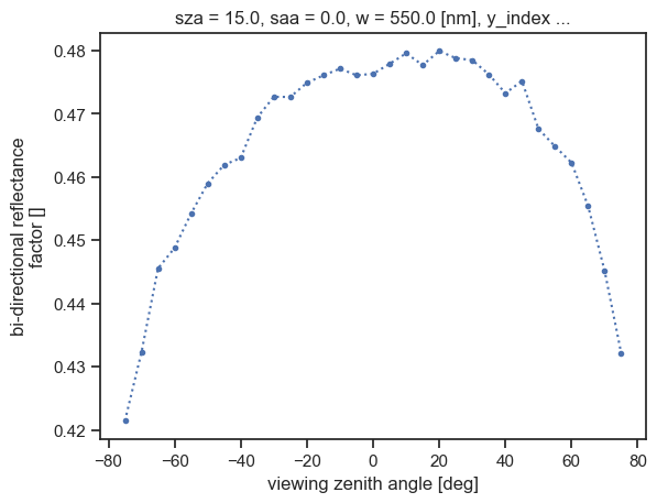214 ... 0.4321
    irradiance  (sza, saa, w) float64 8B 1.843

xarray.Dataset

• Dimensions:
  • sza: 1
  • saa: 1
  • w: 1
  • y_index: 1
  • x_index: 31
• Coordinates: (9)
  • sza
    (sza)
    float64
    15.0

    array([15.])

  • saa
    (saa)
    float64
    0.0

    array([0.])

  • w
    (w)
    float64
    550.0

    standard_name :

    radiation_wavelength

    long_name :

    wavelength

    units :

    nm

    array([550.])

  • y_index
    (y_index)
    int64
    0

    array([0])

  • y
    (y_index)
    float64
    0.0

    long_name :

    film height coordinate

    array([0.])

  • x_index
    (x_index)
    int64
    0 1 2 3 4 5 6 ... 25 26 27 28 29 30

    array([ 0,  1,  2,  3,  4,  5,  6,  7,  8,  9, 10, 11, 12, 13, 14, 15, 16, 17,
           18, 19, 20, 21, 22, 23, 24, 25, 26, 27, 28, 29, 30])

  • x
    (x_index)
    float64
    0.0 0.03333 0.06667 ... 0.9667 1.0

    long_name :

    film width coordinate

    array([0.        , 0.03333333, 0.06666667, 0.1       , 0.13333333,
           0.16666667, 0.2       , 0.23333333, 0.26666667, 0.3       ,
           0.33333333, 0.36666667, 0.4       , 0.43333333, 0.46666667,
           0.5       , 0.53333333, 0.56666667, 0.6       , 0.63333333,
           0.66666667, 0.7       , 0.73333333, 0.76666667, 0.8       ,
           0.83333333, 0.86666667, 0.9       , 0.93333333, 0.96666667,
           1.        ])

  • vza
    (x_index, y_index)
    int64
    -75 -70 -65 -60 -55 ... 60 65 70 75

    standard_name :

    viewing_zenith_angle

    long_name :

    viewing zenith angle

    units :

    deg

    array([[-75],
           [-70],
           [-65],
           [-60],
           [-55],
           [-50],
           [-45],
           [-40],
           [-35],
           [-30],
           [-25],
           [-20],
           [-15],
           [-10],
           [ -5],
           [  0],
           [  5],
           [ 10],
           [ 15],
           [ 20],
           [ 25],
           [ 30],
           [ 35],
           [ 40],
           [ 45],
           [ 50],
           [ 55],
           [ 60],
           [ 65],
           [ 70],
           [ 75]])

  • vaa
    (x_index, y_index)
    int64
    0 0 0 0 0 0 0 0 ... 0 0 0 0 0 0 0 0

    standard_name :

    viewing_azimuth_angle

    long_name :

    viewing azimuth angle

    units :

    deg

    array([[0],
           [0],
           [0],
           [0],
           [0],
           [0],
           [0],
           [0],
           [0],
           [0],
           [0],
           [0],
           [0],
           [0],
           [0],
           [0],
           [0],
           [0],
           [0],
           [0],
           [0],
           [0],
           [0],
           [0],
           [0],
           [0],
           [0],
           [0],
           [0],
           [0],
           [0]])

• Data variables: (4)
  • radiance
    (w, y_index, x_index, saa, sza)
    float64
    0.2472 0.2536 ... 0.2611 0.2535

    standard_name :

    radiance

    long_name :

    radiance

    units :

    W / m ** 2 / nm / sr

    array([[[[[0.24723813]],
    
             [[0.25361034]],
    
             [[0.26137891]],
    
             [[0.26327869]],
    
             [[0.26647818]],
    
             [[0.26926863]],
    
             [[0.27098596]],
    
             [[0.27163118]],
    
             [[0.27538159]],
    
             [[0.27729732]],
    
    ...
    
             [[0.28069866]],
    
             [[0.2793811 ]],
    
             [[0.27763408]],
    
             [[0.27875727]],
    
             [[0.27432185]],
    
             [[0.27270064]],
    
             [[0.27118155]],
    
             [[0.26717073]],
    
             [[0.26114973]],
    
             [[0.25352755]]]]])

  • brdf
    (w, y_index, x_index, saa, sza)
    float64
    0.1341 0.1376 ... 0.1417 0.1376

    standard_name :

    brdf

    long_name :

    bi-directional reflection distribution function

    units :

    1 / sr

    array([[[[[0.13414367]],
    
             [[0.13760103]],
    
             [[0.14181602]],
    
             [[0.14284678]],
    
             [[0.14458272]],
    
             [[0.14609673]],
    
             [[0.1470285 ]],
    
             [[0.14737858]],
    
             [[0.14941343]],
    
             [[0.15045285]],
    
    ...
    
             [[0.15229831]],
    
             [[0.15158344]],
    
             [[0.15063556]],
    
             [[0.15124497]],
    
             [[0.14883845]],
    
             [[0.14795883]],
    
             [[0.14713462]],
    
             [[0.14495847]],
    
             [[0.14169167]],
    
             [[0.13755611]]]]])

  • brf
    (w, y_index, x_index, saa, sza)
    float64
    0.4214 0.4323 ... 0.4451 0.4321

    standard_name :

    brf

    long_name :

    bi-directional reflectance factor

    units :

    array([[[[[0.42142477]],
    
             [[0.4322864 ]],
    
             [[0.44552816]],
    
             [[0.44876639]],
    
             [[0.45422001]],
    
             [[0.45897642]],
    
             [[0.46190366]],
    
             [[0.46300345]],
    
             [[0.46939615]],
    
             [[0.47266155]],
    
    ...
    
             [[0.47845924]],
    
             [[0.47621342]],
    
             [[0.47323558]],
    
             [[0.47515009]],
    
             [[0.46758979]],
    
             [[0.46482637]],
    
             [[0.46223705]],
    
             [[0.45540048]],
    
             [[0.44513751]],
    
             [[0.43214528]]]]])

  • irradiance
    (sza, saa, w)
    float64
    1.843

    standard_name :

    horizontal_solar_irradiance_per_unit_wavelength

    long_name :

    horizontal spectral irradiance

    units :

    W / m ** 2 / nm

    array([[[1.84308457]]])

• Indexes: (5)
  • sza
    PandasIndex

    PandasIndex(Index([15.0], dtype='float64', name='sza'))

  • saa
    PandasIndex

    PandasIndex(Index([0.0], dtype='float64', name='saa'))

  • w
    PandasIndex

    PandasIndex(Index([550.0], dtype='float64', name='w'))

  • y_index
    PandasIndex

    PandasIndex(Index([0], dtype='int64', name='y_index'))

  • x_index
    PandasIndex

    PandasIndex(Index([ 0,  1,  2,  3,  4,  5,  6,  7,  8,  9, 10, 11, 12, 13, 14, 15, 16, 17,
           18, 19, 20, 21, 22, 23, 24, 25, 26, 27, 28, 29, 30],
          dtype='int64', name='x_index'))

• Attributes: (0)

We can see that a brf variable is present. To visualise it, we create a Matplotlib figure and plot the BRF data, using xarray’s built-in plotting interface. By passing the x coordinate in the plotting method, we choose which coordinate to plot against. We also set markers and line style to visualise sample location more precisely.

fig = plt.figure()
results.brf.plot(x="vza", linestyle=":", marker=".");

---

Final words

Bravo! You just completed your first Eradiate simulation. You can now try and modify it, for instance by changing the sample count (check the effect on the processing time and the Monte Carlo noise in the results) or the zenith angles of the measure.

Further reading

• Molecular atmosphere basics