Go to notebook file

---

%reload_ext eradiate.notebook.tutorials

Last updated: 2024-03-07 15:49 (eradiate v0.25.1.dev31+g2a83b0ba.d20240229)

Problem geometry control

Overview

This tutorial introduces Eradiate’s problem geometry control feature, which allows to select the basic problem geometry (plane-parallel or spherical-shell) for experiments supporting it.

Prerequisites

• How to set up an experiment and run a simulation with Eradiate.

• How to visualise a scene.

What you will learn

• How to select the problem geometry when configuring an experiment.

---

Geometry control interface

We start by activating the IPython extension and importing and aliasing a few useful components. We also select the monochromatic mode.

%load_ext eradiate

import attr
import numpy as np
import xarray as xr
from rich.pretty import pprint
import matplotlib.pyplot as plt

import eradiate
from eradiate import unit_registry as ureg
eradiate.set_mode("mono")

We now set up an experiment simulating radiative transfer for a one-dimensional plane-parallel geometry. This is done with the AtmosphereExperiment class and its geometry parameter.

We will use a perspective camera to visualise clearly the surface. We use an intermediate sample count (spp parameter) to reduce noise a little.

exp_ppa = eradiate.experiments.AtmosphereExperiment(
    geometry="plane_parallel",
    atmosphere={
        "type": "molecular",
        "has_absorption": False,
    },
    measures={
        "type": "perspective",
        "origin": [-1000, 0, 110] * ureg.km,
        "target": [0, 0, 110] * ureg.km,
        "up": [0, 0, 1],
        "film_resolution": (320, 160),
        "spp": 128,
    }
)

Now, we run the simulation and plot the resulting image.

result = eradiate.run(exp_ppa)
result.radiance.squeeze().plot.imshow(
    yincrease=False, robust=True, aspect=2, size=4
)

<matplotlib.image.AxesImage object at 0x7f7e62abe250>

Our surface is a horizontal line, just as we expected. Now, we can define a second experiment, which will be indentical, except for the problem geometry. To achieve this, all we have to do is set the geometry parameter to "spherical_shell":

exp_ssa = eradiate.experiments.AtmosphereExperiment(
    geometry="spherical_shell",
    atmosphere=exp_ppa.atmosphere,
)

We can visualise the settings which were automatically selected. The planet radius is that of Earth, but it can be set to any value by passing directly a SphericalShellGeometry instance as the geometry parameter.

exp_ssa.geometry

SphericalShellGeometry(
    toa_altitude=120.0 km,
    ground_altitude=0.0 km,
    zgrid=ZGrid(
        levels=[0.0 100.0 200.0 ... 119800.0 119900.0 120000.0] m,
        _layers=[50.0 150.0 250.0 ... 119750.0 119850.0 119950.0] m,
        _layer_height=100.0 m,
        _total_height=120000.0 m
    ),
    planet_radius=6378.1 km
)

We also have to update our perspective camera setup because the scene is now based on a sphere centred at (0, 0, 0), and not a rectangular surface. Consequently, we must change where our camera is located and where it is looking.

camera_ppa = exp_ppa.measures[0]
offset = [0, 0, exp_ssa.geometry.planet_radius.m_as(ureg.km)] * ureg.km

exp_ssa = eradiate.experiments.AtmosphereExperiment(
    geometry="spherical_shell",
    atmosphere=exp_ppa.atmosphere,
    measures={
        "type": "perspective",
        "origin": camera_ppa.origin + offset,
        "target": camera_ppa.target + offset,
        "up": camera_ppa.up,
        "film_resolution": camera_ppa.film_resolution,
        "spp": camera_ppa.spp
    }
)

We run the simulation and display the resulting image, on which the curvature of the surface is clearly visible.

result = eradiate.run(exp_ssa)
result.radiance.squeeze().plot.imshow(
    yincrease=False, robust=True, aspect=2, size=4
)

<matplotlib.image.AxesImage object at 0x7f7e6282c8e0>

BRF simulation

Now that we know how to set the surface geometry, let us run a few top-of-atmosphere BRF simulations. We define two also identical experiments, one with a plane-parallel geometry, and the other with a spherical-shell geometry. A good setup to observe the effect of how switching to a spherical-shell geometry is decreases the optical path is to use an abstract example with a non-absorbing atmosphere model and a black surface.

experiments = {}

for geometry in ["plane_parallel", "spherical_shell"]:
    experiments[geometry] = eradiate.experiments.AtmosphereExperiment(
        geometry=geometry,
        atmosphere={
            "type": "molecular",
            "has_scattering": True,
            "has_absorption": False,
        },
        surface={"type": "black"},
        illumination={
            "type": "directional",
            "zenith": 0 * ureg.deg,
        },
        measures={
            "type": "mdistant",
            "construct": "hplane",
            "zeniths": (
                [-88, -87, -86] +
                list(np.arange(-85, 86, 5)) +
                [86, 87, 88]
            ) * ureg.deg,
            "azimuth": 0.0,
            "spp": 100000,
        }
    )

We can now run the simulation.

results = {}
for geometry, experiment in experiments.items():
    results[geometry] = eradiate.run(experiment)

The xarray library makes it very simple to assemble our results into a single dataset. We can then visualise it very conveniently.

ds = xr.concat(list(results.values()), dim="geometry")
ds = ds.assign_coords(geometry=list(results.keys()))
ds.brf.squeeze(drop=True).plot(
    hue="geometry", x="vza", linestyle=":", marker="."
);

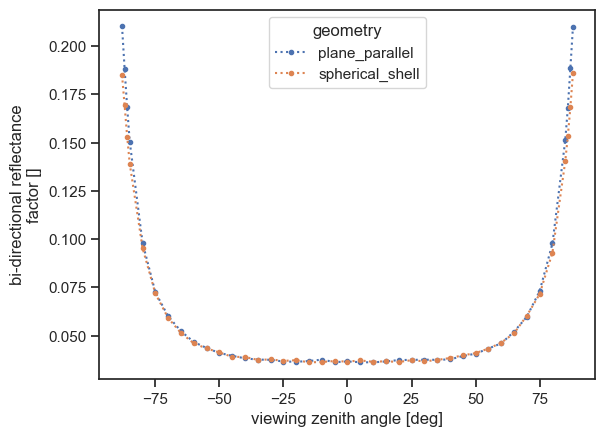
Note how the reduced optical path in the spherical-shell configuration also reduces the amount of light scattered to the sensor, and therefore decreases the recorded radiance.

---

Final words

While the plane-parallel geometry is appropriate in many common situations, it shows its limits at high illumination and viewing angles. You can further explore these effects by using and therefore decreases the recorded radiancemore realistic surface and atmospheric models (you will have to switch to the CKD mode if you want to use the AFGL 1986 profiles).

Further reading

• The PlaneParallelGeometry and SphericalShellGeometry classes allow for advanced geometry control, see their respective documentation pages for further detail.