[1]:
%reload_ext eradiate.tutorials
Last updated: 2025-08-28 18:03 (eradiate v0.31.0.dev1)
Particle layer basics
Overview
In this tutorial, we introduce Eradiate’s particle layer simulation features. We also introduce the general heterogeneous atmosphere container.
Prerequisites
Ability to run and visualize 1D simulations (see First steps with Eradiate).
(Optional but recommended) Ability to configure a molecular atmosphere (see Molecular atmosphere basics).
What you will learn
How to add one or several aerosol layers to a molecular atmosphere.
The particle layer interface
We start by activating the IPython extension and importing and aliasing a few useful components. We also select the CKD mode.
[2]:
%load_ext eradiate
import eradiate
import matplotlib.pyplot as plt
import numpy as np
from eradiate.notebook.tutorials import plot_sigma_t

eradiate.set_mode("ckd")
We alias the eradiate.scenes module and the unit registry for convenience:
[3]:
import eradiate.scenes as ertsc
from eradiate import unit_registry as ureg
The ParticleLayer class is used to configure particle layers. It is parametrised by:
an extent, defined by its bottom and top parameters;
a number of layers (n_layers) the particle layer is discretised;
a particle spatial density distribution (e.g. uniform or gaussian)
an optical thickness value (tau_ref) at a reference wavelength set by its w_ref parameter (by default 550 nm).
We start by creating a particle layer with default parameters:
[4]:
particle_layer_default = ertsc.atmosphere.ParticleLayer()
particle_layer_default
[4]:
ParticleLayer(
    id='atmosphere',
    geometry=PlaneParallelGeometry(
        toa_altitude=120.0 km,
        ground_altitude=0.0 km,
        zgrid=ZGrid(
            levels=[0.0 100.0 200.0 ... 119800.0 119900.0 120000.0] m,
            _layers=[50.0 150.0 250.0 ... 119750.0 119850.0 119950.0] m,
            _layer_height=100.0 m,
            _total_height=120000.0 m
        ),
        width=1000000.0 km
    ),
    scale=None,
    force_majorant=False,
    bottom=0.0 km,
    top=1.0 km,
    distribution=UniformParticleDistribution(bounds=array([0., 1.])),
    w_ref=550 nm,
    tau_ref=0.2,
    dataset=<xarray.Dataset | source='/home/leroyv/.cache/eradiate/installed/eradiate-v0.31.0.dev1/aerosol/govaerts_2021-continental.nc'>,
    has_absorption=True,
    has_scattering=True,
    force_polarized_phase=False,
    particle_shape='spherical',
    _phase=TabulatedPhaseFunction(
        id='phase_atmosphere',
        data=<xarray.DataArray | name='phase', dims=['w', 'mu', 'i', 'j'], source='/home/leroyv/.cache/eradiate/installed/eradiate-v0.31.0.dev1/aerosol/govaerts_2021-continental.nc'>,
        force_polarized_phase=False,
        particle_shape='spherical'
    )
)
We see that our particle_layer_default variable represents an aerosol layer with:
a vertical extent from 0 to 1 km;
a uniform particle density distribution within that extent;
an optical thickness at 550 nm equal to 0.2.
We also note that the geometry field is set to a default suitable for the simulation of a typical atmospheric profile, ranging from 0 to 120 km with a 100 m grid step.
We can now visualize the extinction coefficient using the following convenience function:
[5]:
plot_sigma_t(particle_layer_default, altitude_extent=[0, 2])
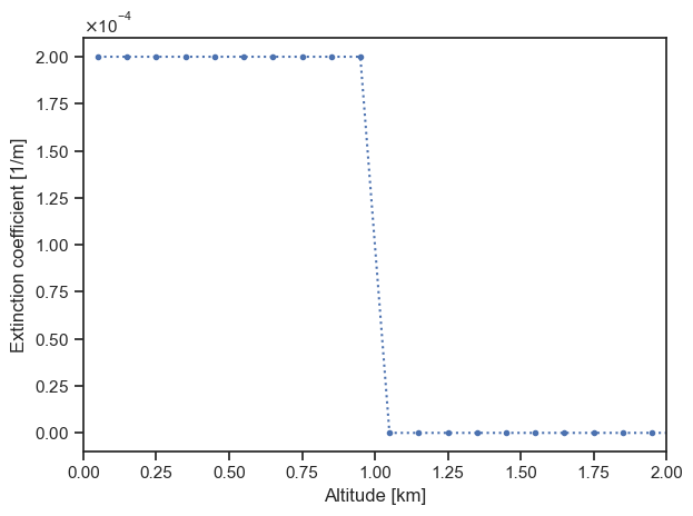
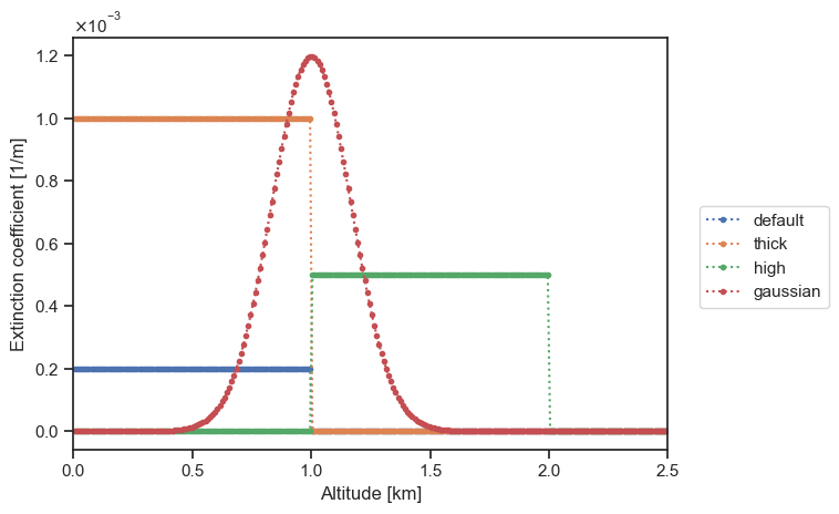
We note that the extinction coefficient drops to 0 above 1 km: the particle layer cover the [0, 1] km region, and the rest of the atmospheric profile consists in a vacuum.
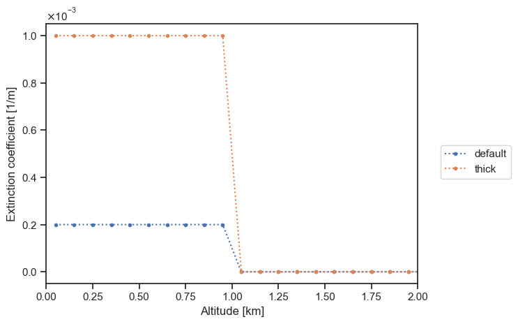
Now, let’s define another particle layer with a different optical thickness:
[6]:
particle_layer_thick = ertsc.atmosphere.ParticleLayer(tau_ref=1.0)
plot_sigma_t(
    particle_layer_default,
    particle_layer_thick,
    labels=["default", "thick"],
    altitude_extent=[0, 2],
)
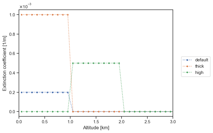
We can also modify the extent of our particle using the bottom and top parameters:
[7]:
particle_layer_high = ertsc.atmosphere.ParticleLayer(
    tau_ref=0.5, bottom=1 * ureg.km, top=2 * ureg.km
)
plot_sigma_t(
    particle_layer_default,
    particle_layer_thick,
    particle_layer_high,
    labels=["default", "thick", "high"],
    altitude_extent=[0, 3],
)
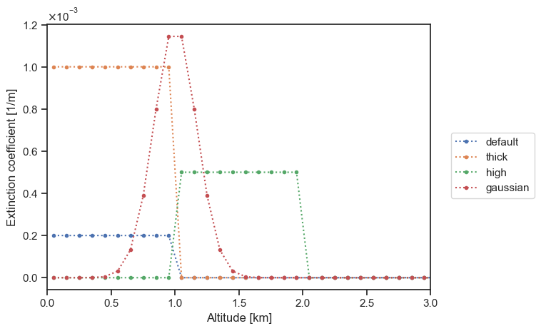
We can vary the particle density distribution within the defined bounds:
[8]:
particle_layer_gaussian = ertsc.atmosphere.ParticleLayer(
    tau_ref=0.5,
    bottom=0.5 * ureg.km,
    top=1.5 * ureg.km,
    distribution="gaussian",
)

plot_sigma_t(
    particle_layer_default,
    particle_layer_thick,
    particle_layer_high,
    particle_layer_gaussian,
    labels=["default", "thick", "high", "gaussian"],
    altitude_extent=[0, 3],
)
Finally, we can modify the altitude grid to allow for a more accurate extinction distribution profile:
[9]:
geometry = ertsc.geometry.PlaneParallelGeometry(
    zgrid=np.arange(0, 10001, 10) * ureg.m,
    toa_altitude=10 * ureg.km,
)

for particle_layer in [
    particle_layer_default,
    particle_layer_thick,
    particle_layer_high,
    particle_layer_gaussian,
]:
    particle_layer.geometry = geometry

plot_sigma_t(
    particle_layer_default,
    particle_layer_thick,
    particle_layer_high,
    particle_layer_gaussian,
    labels=["default", "thick", "high", "gaussian"],
    altitude_extent=[0, 2.5],
)
Adding a particle layer to a molecular atmosphere
Although Eradiate can simulate radiative transfer in a single particle layer, realistic use cases rather involve adding a particle layer to a molecular atmosphere. For this, we use the HeterogeneousAtmosphere class. This class acts as a container which can mix a MolecularAtmosphere and an arbitrary number of ParticleLayers.
[10]:
exponential = ertsc.atmosphere.ParticleLayer(
    tau_ref=0.05,
    bottom=0 * ureg.km,
    top=6 * ureg.km,
    distribution="exponential",
)

gaussian = ertsc.atmosphere.ParticleLayer(
    tau_ref=0.02,
    bottom=1 * ureg.km,
    top=2 * ureg.km,
    distribution="gaussian",
)

atmosphere = ertsc.atmosphere.HeterogeneousAtmosphere(
    molecular_atmosphere={"type": "molecular"},
    particle_layers=[exponential, gaussian]
)
We can display the extinction coefficient for the full atmospheric profile and all its components as follows (note that we restrict the view range to the [0, 10] km extent for clarity):
[11]:
plot_sigma_t(
    atmosphere,
    atmosphere.molecular_atmosphere,
    exponential,
    gaussian,
    altitude_extent=(0, 10),
)
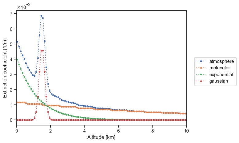
We see on this plot that the various components of the HeterogeneousAtmosphere container are stacked as expected. We also see that the components are all assumed piecewise-constant on their own grid, then regridded on a fine mesh prior to merge.
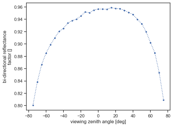
Running the simulation
We can now use this atmosphere definition to run a 1D simulation and compute the top-of-atmosphere BRF:
[12]:
# Show only spectral loop progress
eradiate.config.progress = "spectral_loop"

exp = eradiate.experiments.AtmosphereExperiment(
    surface={"type": "lambertian", "reflectance": 1.0},
    atmosphere=atmosphere,
    illumination={"type": "directional", "zenith": 30.0, "azimuth": 0.0},
    measures={
        "type": "mdistant",
        "construct": "hplane",
        "zeniths": np.arange(-75, 76, 5),
        "azimuth": 0.0,
        "srf": {"type": "multi_delta", "wavelengths": 550.0 * ureg.nm},  # Run the simulation for the 550 nm bin
        "spp": 10000,
    },
)
result = eradiate.run(exp)
result
[12]:
<xarray.Dataset> Size: 2kB
Dimensions:     (sza: 1, saa: 1, w: 1, y_index: 1, x_index: 31)
Coordinates:
  * sza         (sza) float64 8B 30.0
  * saa         (saa) float64 8B 0.0
  * w           (w) float64 8B 551.0
  * y_index     (y_index) int64 8B 0
    y           (y_index) float64 8B 0.0
  * x_index     (x_index) int64 248B 0 1 2 3 4 5 6 7 ... 23 24 25 26 27 28 29 30
    x           (x_index) float64 248B 0.0 0.03333 0.06667 ... 0.9333 0.9667 1.0
    vza         (x_index, y_index) int64 248B -75 -70 -65 -60 ... 60 65 70 75
    vaa         (x_index, y_index) int64 248B 0 0 0 0 0 0 0 0 ... 0 0 0 0 0 0 0
    bin_wmin    (w) float64 8B 549.5
    bin_wmax    (w) float64 8B 552.5
Data variables:
    radiance    (w, y_index, x_index, saa, sza) float64 248B 0.4179 ... 0.4189
    brdf        (w, y_index, x_index, saa, sza) float64 248B 0.2557 ... 0.2563
    brf         (w, y_index, x_index, saa, sza) float64 248B 0.8033 ... 0.8053
irradiance (sza, saa, w) float64 8B 1.634And we can plot the computed TOA BRF:
[13]:
with plt.rc_context({"lines.marker": ".", "lines.linestyle": ":"}):
    result.brf.squeeze(drop=True).plot(x="vza")
Final words
This quick introduction provides just an overview of how particle layers are parametrised. In particular, particle radiative property datasets (the dataset parameter of the ParticleLayer constructor) are not (yet) covered by this tutorial. Until this is done, you can have a look in the resources/data/spectra/particles and explore those datasets.
Further reading
List of available particle density distributions:
particle_distribution_factoryParticle optical property data guide: Aerosol / particle single-scattering radiative properties