[1]:
%reload_ext eradiate.notebook.tutorials
Last updated: 2024-03-07 15:48 (eradiate v0.25.1.dev31+g2a83b0ba.d20240229)
Post-processing pipelines#
Overview
Eradiate provides, for each experiment type, a default post-processing pipeline. However, you might want to perform tasks that go beyond what the default pipeline can achieve, such as applying several spectral response functions to a recorded signal. This tutorial explains how to intercept post-processing pipeline data and how to apply pipeline steps manually.
Prerequisites
Basic knowledge of the Eradiate workflow (see First steps with Eradiate).
Prior knowledge of the Hamilton library is useful but not required.
What you will learn
How to inspect post-processing pipelines.
How to retrieve arbitrary data from the pipeline.
How to build a custom post-processing chain.
Imports#
As for all tutorials the first step is to import all necessary classes and create aliases for convenience:
[2]:
%load_ext eradiate

import numpy as np
import pandas as pd
import xarray as xr
import matplotlib.pyplot as plt
import eradiate
eradiate.set_mode("ckd")
eradiate.config.progress = "spectral_loop"

import eradiate.scenes as ertsc
from eradiate import unit_registry as ureg
Visualizing the pipeline#
We set up a basic simulation to visualize its post-processing pipeline:
[3]:
exp = eradiate.experiments.AtmosphereExperiment(
    illumination={
        "type": "directional",
        "zenith": 30,
    },
    measures={
        "type": "mdistant",
        "construct": "hplane",
        "azimuth": 0.0,
        "zeniths": np.arange(-75.0, 76.0, 5.0),
        "srf": "sentinel_2a-msi-3",
        "spp": 10000,
    }
)
Now, we can use the pipeline() method to fetch the experiment’s post-processing pipeline, which is a Hamilton Driver object:
[4]:
drv = exp.pipeline(0)
The Driver defines how post-processing operations chain with each other, builds a graph to represent the pipeline and specifies the input, output and intermediate data handled during workflow execution. The Driver instance has a method to display its internal graph:
[5]:
drv.display_all_functions()
[5]:

On this graph, we can see all the functions that will be executed during post-processing, as well as the inputt and configuration variables, together with their corresponding data types. We can also list the variables as a table:
[6]:
eradiate.pipelines.list_variables(drv, as_table=True)
[6]:
┏━━━━━━━━━━━━━━━━━━━━━━━━━━━━━━━┳━━━━━━━━━━━━━━┳━━━━━━━┓
┃ Name                          ┃ Type         ┃ Input ┃
┡━━━━━━━━━━━━━━━━━━━━━━━━━━━━━━━╇━━━━━━━━━━━━━━╇━━━━━━━┩
│ angles                        │ ndarray      │ x     │
│ bitmaps                       │ dict         │ x     │
│ illumination                  │ Illumination │ x     │
│ spectral_set                  │ SpectralSet  │ x     │
│ srf                           │ Spectrum     │ x     │
│ bidirectional_reflectance     │ dict         │       │
│ bidirectional_reflectance_srf │ dict         │       │
│ brdf                          │ DataArray    │       │
│ brdf_srf                      │ DataArray    │       │
│ brf                           │ DataArray    │       │
│ brf_srf                       │ DataArray    │       │
│ extract_irradiance            │ dict         │       │
│ gather_bitmaps                │ dict         │       │
│ irradiance                    │ DataArray    │       │
│ irradiance_srf                │ DataArray    │       │
│ radiance                      │ DataArray    │       │
│ radiance_raw                  │ DataArray    │       │
│ radiance_srf                  │ DataArray    │       │
│ solar_angles                  │ Dataset      │       │
│ spectral_response             │ DataArray    │       │
│ spp                           │ DataArray    │       │
│ viewing_angles                │ Dataset      │       │
│ weights_raw                   │ DataArray    │       │
└───────────────────────────────┴──────────────┴───────┘
Upon pipeline execution, Hamilton builds an execution graph from the global one we just displayed. For that purpose, it needs the outputs requested by the user. We can pick output names from the table above to see what happens if the driver is requested the irradiance and radiance products. In order to visualize execution, Hamilton also requires that we provide inputs: to start with, we provide a fake input dictionary.
Note
The list of inputs may look like it was magically made up; it was not! If you try and call the visualize_execution() method with missing input, an exception will be raised and it will include the list of missing inputs.
[7]:
drv.visualize_execution(
    final_vars=["radiance", "irradiance"],
    inputs={"angles": None, "bitmaps": None, "illumination": None, "spectral_set": None},
    orient="TD",
)
[7]:

We can see that Hamilton pruned the global graph to execute only the nodes that will contribute to the requested variables. We can also request intermediate outputs in a similar way:
[8]:
drv.visualize_execution(
    final_vars=["radiance", "irradiance", "solar_angles"],
    inputs={"angles": None, "bitmaps": None, "illumination": None, "spectral_set": None},
    orient="TD",
)
[8]:

With this, we have the basic tool to understand which are the input and output variable of the post-processing pipeline. Now, let’s see how to use it.
Running the pipeline#
If you use the recommended workflow to run an experiment, the post-processing pipeline execution is performed automatically. A list of experiment-specific post-processing outputs are automatically assembled into an xarray dataset.
[9]:
eradiate.run(exp)
[9]:
<xarray.Dataset> Size: 6kB
Dimensions:         (sza: 1, saa: 1, w: 6, y_index: 1, x_index: 31)
Coordinates:
  * sza             (sza) int64 8B 30
  * saa             (saa) float64 8B 0.0
  * w               (w) float64 48B 545.0 555.0 565.0 575.0 585.0 595.0
  * y_index         (y_index) int64 8B 0
    y               (y_index) float64 8B 0.0
  * x_index         (x_index) int64 248B 0 1 2 3 4 5 6 ... 24 25 26 27 28 29 30
    x               (x_index) float64 248B 0.0 0.03333 0.06667 ... 0.9667 1.0
    vza             (x_index, y_index) float64 248B -75.0 -70.0 ... 70.0 75.0
    vaa             (x_index, y_index) float64 248B 0.0 0.0 0.0 ... 0.0 0.0 0.0
    bin_wmin        (w) float64 48B 540.0 550.0 560.0 570.0 580.0 590.0
    bin_wmax        (w) float64 48B 550.0 560.0 570.0 580.0 590.0 600.0
Data variables:
    radiance        (w, y_index, x_index, saa, sza) float64 1kB 0.3366 ... 0....
    radiance_srf    (y_index, x_index, saa, sza) float64 248B 0.3275 ... 0.3648
    irradiance_srf  (sza, saa) float64 8B 1.645
    brdf            (w, y_index, x_index, saa, sza) float64 1kB 0.2036 ... 0....
    brf             (w, y_index, x_index, saa, sza) float64 1kB 0.6397 ... 0.672
    brdf_srf        (y_index, x_index, saa, sza) float64 248B 0.1991 ... 0.2218
    brf_srf         (y_index, x_index, saa, sza) float64 248B 0.6256 ... 0.6969
irradiance (sza, saa, w) float64 48B 1.653 1.669 1.619 ... 1.594 1.555We can also decide to trigger the post-processing step manually.
Note
The following code is more or less equivalent to what eradiate.run() does.
[10]:
exp.clear()
exp.process()
exp.postprocess()
exp.results["measure"]
[10]:
<xarray.Dataset> Size: 6kB
Dimensions:         (sza: 1, saa: 1, w: 6, y_index: 1, x_index: 31)
Coordinates:
  * sza             (sza) int64 8B 30
  * saa             (saa) float64 8B 0.0
  * w               (w) float64 48B 545.0 555.0 565.0 575.0 585.0 595.0
  * y_index         (y_index) int64 8B 0
    y               (y_index) float64 8B 0.0
  * x_index         (x_index) int64 248B 0 1 2 3 4 5 6 ... 24 25 26 27 28 29 30
    x               (x_index) float64 248B 0.0 0.03333 0.06667 ... 0.9667 1.0
    vza             (x_index, y_index) float64 248B -75.0 -70.0 ... 70.0 75.0
    vaa             (x_index, y_index) float64 248B 0.0 0.0 0.0 ... 0.0 0.0 0.0
    bin_wmin        (w) float64 48B 540.0 550.0 560.0 570.0 580.0 590.0
    bin_wmax        (w) float64 48B 550.0 560.0 570.0 580.0 590.0 600.0
Data variables:
    radiance        (w, y_index, x_index, saa, sza) float64 1kB 0.3252 ... 0....
    radiance_srf    (y_index, x_index, saa, sza) float64 248B 0.3239 ... 0.3634
    irradiance_srf  (sza, saa) float64 8B 1.645
    brdf            (w, y_index, x_index, saa, sza) float64 1kB 0.1967 ... 0....
    brf             (w, y_index, x_index, saa, sza) float64 1kB 0.6181 ... 0....
    brdf_srf        (y_index, x_index, saa, sza) float64 248B 0.1969 ... 0.2209
    brf_srf         (y_index, x_index, saa, sza) float64 248B 0.6187 ... 0.6941
irradiance (sza, saa, w) float64 48B 1.653 1.669 1.619 ... 1.594 1.555Finally, we can decide to run the post-processing pipeline manually:
[11]:
i_measure = 0
drv = exp.pipeline(i_measure)
outputs = ["brf"]
inputs = {
    "angles": exp.measures[i_measure].viewing_angles.m_as("deg"),
    "illumination": exp.illumination,
    "bitmaps": exp.measures[i_measure].mi_results,
    "spectral_set": exp.spectral_set[i_measure]
}
results = drv.execute(final_vars=outputs, inputs=inputs)
The result dictionary maps output variable names with their computed values. In our case, we have a single "brf" field:
[12]:
results["brf"]
[12]:
<xarray.DataArray 'brf' (w: 6, y_index: 1, x_index: 31, saa: 1, sza: 1)> Size: 1kB
0.6181 0.6287 0.6116 0.6099 0.597 0.5911 ... 0.6648 0.6627 0.6853 0.6857 0.6727
Coordinates:
  * sza       (sza) int64 8B 30
  * saa       (saa) float64 8B 0.0
  * w         (w) float64 48B 545.0 555.0 565.0 575.0 585.0 595.0
  * y_index   (y_index) int64 8B 0
    y         (y_index) float64 8B 0.0
  * x_index   (x_index) int64 248B 0 1 2 3 4 5 6 7 8 ... 23 24 25 26 27 28 29 30
    x         (x_index) float64 248B 0.0 0.03333 0.06667 ... 0.9333 0.9667 1.0
    vza       (x_index, y_index) float64 248B -75.0 -70.0 -65.0 ... 70.0 75.0
    vaa       (x_index, y_index) float64 248B 0.0 0.0 0.0 0.0 ... 0.0 0.0 0.0
    bin_wmin  (w) float64 48B 540.0 550.0 560.0 570.0 580.0 590.0
    bin_wmax  (w) float64 48B 550.0 560.0 570.0 580.0 590.0 600.0
Attributes:
    standard_name:  brf
    long_name:      bi-directional reflectance factor
units: This spectral radiance array can then be processed and plotted using regular xarray facilities:
[13]:
fig, axs = plt.subplots(1, 2, figsize=(8, 4), sharey=True, layout="constrained")
brf = results["brf"]

# Slice along the spectral dimension to get the reflectance for the bin closest to 550 nm
brf_550 = brf.sel(w=550, method="nearest")
brf_550.squeeze(drop=True).plot(ax=axs[0], x="vza")
axs[0].set_title(f"wavelength = {float(brf_550.w)} nm")
axs[0].set_ylabel("brf [−]")

# Select along the viewing angle dimension to get the reflectance at the nadir view
brf_nadir = brf.where(brf.vza == 0.0, drop=True)
brf_nadir.squeeze(drop=True).plot(ax=axs[1])
axs[1].set_title(f"vza = {float(brf_nadir.vza)}°")
axs[1].set_ylabel("")

fig.suptitle(f"sza = {float(brf.sza)}°, saa = {float(brf.saa)}°")
plt.show()
plt.close()
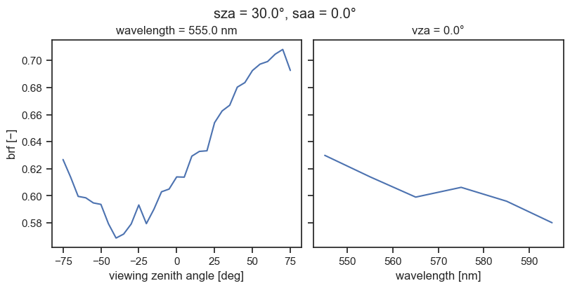
Note that this type of manual operation is usually unnecessary, because the default pipeline will run very quickly and should contain all relevant output variables.
Running custom post-processing operations#
So far, we have been manipulating manually the default post-processing pipeline. Sometimes, however, we might want to do more than what this default pipeline can do. While writing a custom pipeline is possible, it is most often an unnecessary time investment, and we have a much simpler approach to build a custom, single-use post-processing chain. In this section, we will collect intermediate data and apply post-processing routines directly to build our customized output dataset.
As a supporting case, we consider a simulation in which we want to see what two similar instruments observing the same target will record. There are several ways to achieve this, listed here in increasing order of efficiency:
Set up two full-fledged experiments and run the Monte Carlo ray tracing simulation twice. This scenario is the most wasteful because it repeats all steps (experiment pre-processing, processing and post-processing) twice.
Set up a single experiment with two measures. This scenario wastes a little less computational time because it repeats only the ray tracing simulation.
Set up a single experiment covering the union of the spectral range covered by both sensors, extract the spectral signal and apply the spectral response function of both instruments as a custom post-processing step. This is the most efficient method.
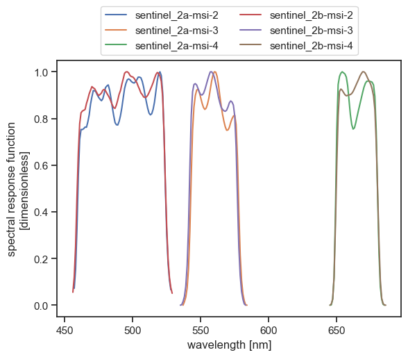
We will see now how to implement method 3. We will simulate a signal recorded by the MSI instruments onboard Sentinel-2A and Sentinel–2B (bands 2, 3 and 4). Let us first have a look at their spectral response functions:
[14]:
bands = [
    "sentinel_2a-msi-2",
    "sentinel_2a-msi-3",
    "sentinel_2a-msi-4",
    "sentinel_2b-msi-2",
    "sentinel_2b-msi-3",
    "sentinel_2b-msi-4",
]

srf_ds = {
    band: eradiate.data.load_dataset(f"spectra/srf/{band}.nc")
    for band in bands
}

fig, ax = plt.subplots(1, 1)
for band, ds in srf_ds.items():
    ds.srf.plot(label=band, ax=ax)
plt.legend(ncol=2, loc="lower center", bbox_to_anchor=(0.5, 1.0))
plt.show()
plt.close()
We can easily extract the bounds of the wavelength domain we should cover:
[15]:
df = pd.DataFrame(
    {
        band: {"wmin": float(ds.w.min()), "wmax": float(ds.w.max())}
        for band, ds in srf_ds.items()
    }
).T
print(f"wmin = {df.wmin.min()}")
print(f"wmax = {df.wmax.max()}")
wmin = 456.0
wmax = 686.0
We use this information to configure define a fictitious SRF which will let the experiment know that we want to process a given interval without apply a particular spectral response function. The simplest way to achieve this is to use the MultiDeltaSpectrum class with many wavelengths in the [\(\lambda_\mathrm{min}\), \(\lambda_\mathrm{max}\)] interval. As explained in the Spectral discretization guide, each wavelength specified in the MultiDeltaSpectrum definition will be used to activate the relevant bin in the spectral discretization. For safety, we use a fairly dense wavelength list (with 1 nm spacing), which we know will be more dense than the spectral discretization. This density would have to be inscreased if we would use a high-resolution atmospheric dataset. We also take a bit of margin on the bounds and set them to 450 nm and 690 nm.
Note
For simplicity, we are here performing the simulation on a connected spectral domain. This makes data processing and plotting simpler, but it is also suboptimal. Ideally, we would use an unconnected spectral domain specification:
srf = {
    "type": "multi_delta",
    "wavelengths": np.concatenate(
        (
            np.arange(450.0, 590.0, 1.0) * ureg.nm, # Bands 2 and 3
            np.arange(640.0, 690.0, 1.0) * ureg.nm, # Band 4
        )
    ),
}
Our minimal experiment setup and run looks like this:
[16]:
exp = eradiate.experiments.AtmosphereExperiment(
    illumination={
        "type": "directional",
        "zenith": 30,
    },
    measures={
        "type": "mdistant",
        "construct": "hplane",
        "azimuth": 0.0,
        "zeniths": np.arange(-75.0, 76.0, 5.0),
        "srf": {
            "type": "multi_delta",
            "wavelengths": np.arange(450.0, 690.0, 1.0) * ureg.nm
        },
        "spp": 10000,
    }
)
result = eradiate.run(exp)
result
[16]:
<xarray.Dataset> Size: 20kB
Dimensions:     (sza: 1, saa: 1, w: 24, y_index: 1, x_index: 31)
Coordinates:
  * sza         (sza) int64 8B 30
  * saa         (saa) float64 8B 0.0
  * w           (w) float64 192B 455.0 465.0 475.0 485.0 ... 665.0 675.0 685.0
  * y_index     (y_index) int64 8B 0
    y           (y_index) float64 8B 0.0
  * x_index     (x_index) int64 248B 0 1 2 3 4 5 6 7 ... 23 24 25 26 27 28 29 30
    x           (x_index) float64 248B 0.0 0.03333 0.06667 ... 0.9333 0.9667 1.0
    vza         (x_index, y_index) float64 248B -75.0 -70.0 -65.0 ... 70.0 75.0
    vaa         (x_index, y_index) float64 248B 0.0 0.0 0.0 0.0 ... 0.0 0.0 0.0
    bin_wmin    (w) float64 192B 450.0 460.0 470.0 480.0 ... 660.0 670.0 680.0
    bin_wmax    (w) float64 192B 460.0 470.0 480.0 490.0 ... 670.0 680.0 690.0
Data variables:
    radiance    (w, y_index, x_index, saa, sza) float64 6kB 0.3825 ... 0.2562
    brdf        (w, y_index, x_index, saa, sza) float64 6kB 0.2193 ... 0.2003
    brf         (w, y_index, x_index, saa, sza) float64 6kB 0.6888 ... 0.6294
irradiance (sza, saa, w) float64 192B 1.744 1.751 1.831 ... 1.309 1.279Since we used a MultiDeltaSpectrum to specify the instrument’s SRF, only the spectral radiance product is available in the result dataset. Let’s post-process it manually and apply the spectral response function manually. For that purpose, we use the apply_spectral_response() function, which takes as parameters the SRF as an InterpolatedSpectrum, and the radiance data array. The SRF object has to be created manually, and we automate this with a short function:
[17]:
from eradiate.scenes.spectra import InterpolatedSpectrum

# We need to create Eradiate Spectrum instances representing the SRF from the datasets
def srf_spectrum(ds):
    w = ureg.Quantity(ds.w.values, ds.w.attrs["units"])
    srf = ds.data_vars["srf"].values
    return InterpolatedSpectrum(quantity="dimensionless", wavelengths=w, values=srf)
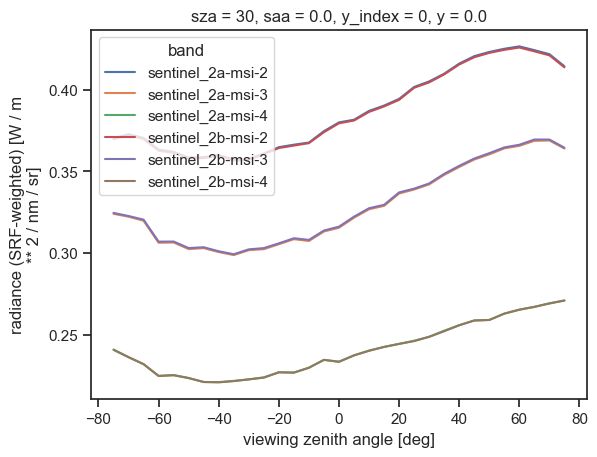
We now proceed with the post-processing operation and aggregate the results into a single data array, each radiance array being indexed on a new band dimension:
[18]:
from eradiate.pipelines.logic import apply_spectral_response

radiances_srf = []

for band in bands:
    srf = srf_spectrum(srf_ds[band])
    radiances_srf.append(apply_spectral_response(result.radiance, srf))

# Now, we concatenate all of these into a data array for convenience
radiance_srf = xr.concat(radiances_srf, dim="band").assign_coords({"band": bands})
radiance_srf
[18]:
<xarray.DataArray 'radiance_srf' (band: 6, y_index: 1, x_index: 31, saa: 1,
                                  sza: 1)> Size: 1kB
0.3703 0.3728 0.3705 0.3633 0.3619 0.3585 ... 0.2628 0.2652 0.267 0.269 0.2709
Coordinates:
  * sza      (sza) int64 8B 30
  * saa      (saa) float64 8B 0.0
  * y_index  (y_index) int64 8B 0
    y        (y_index) float64 8B 0.0
  * x_index  (x_index) int64 248B 0 1 2 3 4 5 6 7 8 ... 23 24 25 26 27 28 29 30
    x        (x_index) float64 248B 0.0 0.03333 0.06667 ... 0.9333 0.9667 1.0
    vza      (x_index, y_index) float64 248B -75.0 -70.0 -65.0 ... 70.0 75.0
    vaa      (x_index, y_index) float64 248B 0.0 0.0 0.0 0.0 ... 0.0 0.0 0.0 0.0
  * band     (band) <U17 408B 'sentinel_2a-msi-2' ... 'sentinel_2b-msi-4'
Attributes:
    standard_name:  radiance_srf
    long_name:      radiance (SRF-weighted)
units: W / m ** 2 / nm / srAnd we can finally plot the resulting dataset using xarray’s built-in plotting routines:
[19]:
radiance_srf.plot(hue="band", x="vza")
plt.show()
plt.close()
Final words#
We have covered the basics on how to perform automatic and manual post-processing. For simplicity, we did not perform a realistic simulation nor address a practical use-case; to go further you can:
Make the simulation more realistic by adding an atmosphere (see the Molecular atmosphere basics and Particle layer basics).
Increase the sample count to reduce the noise in the simulated signal.
In the manual post-processing section, you can compute the BRDF and BRF using the
compute_bidirectional_reflectance()function. You will first need to apply the SRF to the irradiance spectrum in a way similar to what we did for radiance.
Further reading#
The
eradiate.pipelinesreference API documentation, and in particular theeradiate.pipelines.logicmodule which contains all post-processing operation logic.The Spectral discretization guide will help you understand how the instrument spectral response atmospheric absorption data are used to determine the spectral discretization of the simulation.
If you are interested in diving deeper into our post-processing pipeline internals, the Hamilton documentation is a useful source of information.